## here() starts at C:/Work/Research/grainnemcguire.github.io
## Loading required package: Matrix
## Loaded glmnet 4.1-7
## Loading required package: viridisLite
##
## Attaching package: 'viridis'
## The following object is masked from 'package:scales':
##
##     viridis_pal
## Loading required package: foreach
## Loading required package: iterators
## Loading required package: parallelIntroduction
In Taylor & McGuire (2022), Greg Taylor and I looked at using the Lasso, together with Bayesian model averaging and the bootstrap procedure, to estimate internal model structure error in claims reserving. The paper contains the full details of the statistical framework used, so please refer to that for details of the approach.
In this article, or tutorial, what I’d like to share are the details of our bootstrapping approach which was behind the numerical results we discuss in Section 7 of the paper. This is because we consider that our approach tackles a number of practical problems faced by reserving actuaries:
Reserving actuaries must set uncertainty ranges on their reserves. Our approach estimates a number of components of forecast error - while our particular focus was on Internal Model Structure Error (refer to the discussion in Section 3 of the paper for definitions), we are also able to estimate parameter error as a by-product and process error as a straightforward bolt-on to the main process.
Our estimation of model error relies on the model set produced by the Lasso process - the set of models returned of varying complexities. We use Bayesian model averaging to combine these models, but this requires a prior on each model. In the Lasso framework, the prior falls naturally out of the penalty values, or \(\lambda\) parameters used to produce the model set.
The number of models within the Lasso model set is too sparse for reliable estimates of model error, so we use bootstrapping to augment the model set. We show how to bootstrap using a model produced by a Lasso. Furthermore, there are additional challenges in bootstrapping any model that extrapolates into future time periods in that models may display reasonable performance on past time periods, but extrapolate wildly into the future. This is an issue with any reserving model, but is magnified for machine learning models which do not have the same degree of curation to remove model terms that lead to wild behaviour.
In the paper used synthetic data sets in our examples since we were then able to control the complexity of experience within these and better understand the behaviour of model error in that context. Each data set was a 40x40 triangle of aggregate claims payments. However the computational requirements to run each of these are not particularly well-suited to a tutorial example - for example, a recent run of 500 bootstraps for one of the data sets took about 80 minutes using 10 parallel processes on a 16 core linux machine. So for this tutorial I’ve returned to the 10x10 aggregate triangle data we used in our CAS monograph, Stochastic Loss Reserving using Generalized Linear Models. As well as being smaller, we have analysed the data in detail and understand it well. My earlier post discusses this data set in more detail, so please refer to that and the monograph itself for further details.
However, the same code is used in both examples and I will be adding a link to a notebook set up to run the synthetic data examples in due course, so that if you have the grunt power available to you, you can run the synthetic examples if you like (but note that the parallelisation used only works on linux machines - you will need to edit the code to run on windows machines). In the meantime, I suggest you try things on the smaller data set first.
You can download this file as a quarto notebook here.
Pre-requisites
- This builds on the modelling approach in Self-Assembling Insurance Claim Models Using Regularized Regression and Machine Learning, so you may need to consult that paper if you are unfamiliar with it.
- An earlier article works through the details of the model fitting in R.
- The code underlying this is reasoanbly complex and is contained in functions in _functions.R. To really dig into the details of what’s going on, you may need to look at the R code.
R Setup
First I set up my R environment:
- Packages used (see bottom of this article for package versions). One thing I recommend is to check you have a recent version of glmnet (4.1-4 or later) since the package was changed to use C++ at that point leading to spped-ups in runtimes.
- colours and ggplot2 theme settings
- Functions used to run the code - the main parts of the code are sitting in the file _functions.R. Please note that these functions don’t contain much error catching so use them carefully and at your own risk. If you run into problems you may need to use R debugging tools to work out your error.
check for conflicts and resolve if needed (one conflict found).
conflict_scout()
## 1 conflict
## • `viridis_pal()`: viridis and scales
conflict_prefer("viridis_pal", "viridis")
## [conflicted] Will prefer viridis::viridis_pal over any other package.
Next I set up some things I’ll be using below:
main_model: Lasso models are a series of models, and we’ll need to specify one as our preferred or primary model. We use the one labelled aslambda.1sebyglmnet- this is the model within 1 standard deviation of the minimum cross validation error model, often favoured by users as a good trade-off between quality of fit and overfittinglist_dt_filter_paramswhich holds inclusion gates for the bootstrap. There’s more information on these in the paper and below so I’ll defer discussion until then.num_bootstrapsis the number of bootstraps to run. I’ve set this to 100 for the tutorial to keep runtimes manageable, but would recommend more in practice. If you’re running the code, I’d recommend you set it something small like 10 first, just to make sure everything runs, and then increase it to a reasonable number.num_workersandbatchsizerelate to running code in parallel (not done here). Since we run sequentially, setbatchsizeequal tonum_bootstraps
main_model <- "lambda.1se"

# inclusion gates for bootstrap
list_dt_filter_params <- list(
  main = list(
    acc  = data.table(period = c(2, 5, 10), cutoff = c(1.33, 1.25, 1.20)),
    cal  = data.table(period = c(2, 5, 10), cutoff = c(1.10, 1.15, 1.20))
  ))

# set initial wider gates
init_scale <- 1.4
list_dt_filter_params$initial <- list(
  acc = copy(list_dt_filter_params$main$acc)[, cutoff := cutoff * init_scale],
  cal = copy(list_dt_filter_params$main$cal)[, cutoff := cutoff * init_scale]
)

# number of bootstraps
num_bootstraps <- 100
num_workers <- 1  # we run sequentially
batchsize <- num_bootstraps/ num_workers
use_parallel <- FALSE
Data
- The data is located here
- I’ve loaded in the data below using
data.table::fread(). The file path is set using the here package.- I use
data.tablefor all my data manipulations - I’ll aim to describe what each code chunk is doing so even if you’re unfamiliar withdata.tablesyntax, you’ll be able to follow along. - I also use the DT to print out nicely formatted tables using the function
DT::datatable()- this is not related to thedata.tablepackage.
- I use
- I need to do some preparing of the data:
- The csv file only contains past data, but I want past and future so I use
data.table::CJ()to build the full 10x10 skeleton before merging past data on - My model error code requires column names
acc,dev,cal,past_indandpmtsso I make sure I have all the right columns and names after this process.
- The csv file only contains past data, but I want past and future so I use
# edit as needed for your file path
dt_raw <- fread(here("post", "2023-05-04-model-error-example", "_meyersshi.csv"))

# put into matching form
dt <- CJ(acc = 1:10, dev = 1:10)
dt[, cal := acc + dev - 1]
dt[, past_ind := cal <= 10]

dt[ dt_raw, on=.(acc = acc_year, dev = dev_year), pmts := i.incremental]

# Look at the data
datatable(dt)
We can also look at the data graphically too.
p1 <- ggplot(data=dt[past_ind==TRUE,], aes(x=dev, y=log(pmts), colour=as.factor(acc)))+
  geom_line(linewidth = 1)+
  scale_colour_viridis_d(begin=1, end=0, alpha=1)+
  theme(legend.position = "none")+
  labs(title="Each line is an accident quarter", x="Development quarter", y="log(Payments)")+
  NULL

p2 <- ggplot(data=dt[past_ind==TRUE,], aes(x=dev, y=log(pmts), colour=as.factor(cal)))+
  geom_line(linewidth = 1)+
  scale_colour_viridis_d(begin=0, end=1, alpha=1)+
  theme(legend.position = "none")+
  labs(title="Each line is a calendar quarter", x="Development quarter", y="log(Payments)")+
  NULL

p1 + p2   # patchwork to combine plots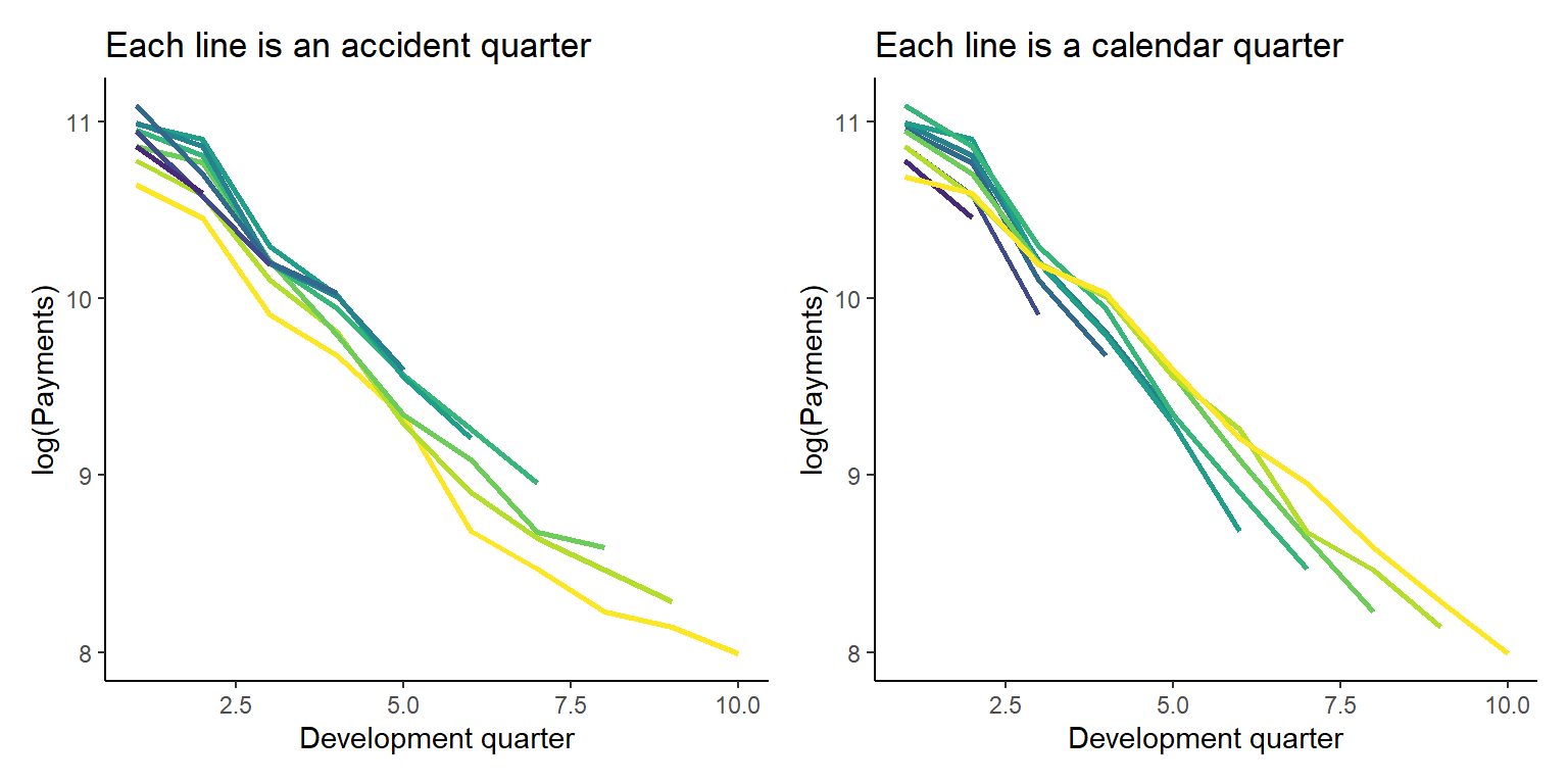
Primary model
Now we built the Lasso model of the data. We use the approach described in our earlier paper, Self-Assembling Insurance Claim Models Using Regularized Regression and Machine Learning. My previous article explains this process in more detail so please refer to that to fill in the gaps - e.g. if you need further details on the basis functions used, how they are defined, scaled etc.
From the CAS monograph work we know that the data are modelled reasonably well by a Chain Ladder model (though our optimal GLM included some accident and development year interactions). So we use this information and only consider accident and development year basis functions. This choice is also motivated by practical reasons - fewer basis functions will make the code run faster, which suits the purposes of this tutorial.
There are a number of tasks we need to do when fitting the model. These include:
- Creating the basis functions to use in the fitting process
- Fitting the model
- Calculating a scale parameter for use in bootstrapping
- Producing model forecasts
- Producing model residuals using the main selected model (lambda.1se in our case) and the scale parameter and looking at some diagnostics
- Specifying the prior
- Producing the initial Bayesian model averaging results from the primary model - this is for interest only - as discussed in our paper, the model set is a bit too sparse to produce reliable estimates of variability, so we need to augment with bootstrapped samples.
First we create list object to hold all of these results.
list_primary <- list()

list_primary$data <- copy(dt)
Basis functions for lasso
Create the basis functions - first create a predictor_obj to hold the settings - e.g. what fundamental variables to include, scaling, what interactions to include. Then use a function to create the basis functions.
As discussed in my earlier article, I’ve gone through a few iterations of the basis function code over the years so what’s in _functions.R may be be a bit different to what’s discussed there.
Set up a predictor object to give information about each of the predictors so that basis functions can be constructed.
The predictor object should contain
num_predictors(2 - acc and dev)predictorsmin- min value of each predictormax- max value of each predictorramp_inc- we build a series of ramp functions and this indicates the increment. Always 1 for things like accident and development periodscaling- this uses theGetScaling()function and applies to the fundamental vector - see the previous articles for more details on scaling
list_primary$predictor_obj <- list()

list_primary$predictor_obj$num_predictors <- 2
list_primary$predictor_obj$predictors <- c("acc", "dev")
list_primary$predictor_obj$min <- c(1, 1)
list_primary$predictor_obj$max <- c(10, 10)
list_primary$predictor_obj$ramp_inc <- c(1, 1)
list_primary$predictor_obj$scaling <- c(GetScaling(dt[past_ind==TRUE, acc]),
GetScaling(dt[past_ind==TRUE, dev])) - We produce a matrix of all the basis functions. For convenience, this is separated into past and future components as well.
- The parameter
int_effects_listis used to specify what interactions to create - in this case all \(I(\text{acc} \ge i) . I(\text(dev) \ge j)\) heaviside interactions.
list_primary$varset <- vector(mode="list", length=3)
names(list_primary$varset) <- c("all", "past", "future")

# all data (NB scaling above based on past data only)
list_primary$varset$all <- GenerateVarset(data = dt,
                                     predictor_object = list_primary$predictor_obj,
                                     main_effects_list = c("acc", "dev"),
                                     int_effects_list = list(c("acc", "dev")))

# past data
list_primary$varset$past <- list_primary$varset$all[dt[, past_ind], ]

# future data
list_primary$varset$future <- list_primary$varset$all[!dt[, past_ind], ]


# look at start of matrix to see what it looks like
list_primary$varset$all[41:46, 1:10]
L_1_999_acc L_2_999_acc L_3_999_acc L_4_999_acc L_5_999_acc L_6_999_acc
[1,] 1.632993 1.224745 0.8164966 0.4082483 0 0
[2,] 1.632993 1.224745 0.8164966 0.4082483 0 0
[3,] 1.632993 1.224745 0.8164966 0.4082483 0 0
[4,] 1.632993 1.224745 0.8164966 0.4082483 0 0
[5,] 1.632993 1.224745 0.8164966 0.4082483 0 0
[6,] 1.632993 1.224745 0.8164966 0.4082483 0 0
L_7_999_acc L_8_999_acc L_9_999_acc L_1_999_dev
[1,] 0 0 0 0.0000000
[2,] 0 0 0 0.4082483
[3,] 0 0 0 0.8164966
[4,] 0 0 0 1.2247449
[5,] 0 0 0 1.6329932
[6,] 0 0 0 2.0412415Lasso fitting
- Here we fit Lasso models using the
glmnetpackage.- Although we use the gamma distribution later in our analysis, we use the Poisson distribution with glmnet when generating our model set since we had convergence issues when using the gamma distribution.
- You’ll notice we do 3 fits:
- The first generates a series of lambda values, but does not do the cross validation
- In the second we lengthen the lambda vector to smaller values to ensure that we do reach the minimum cross validation model and then run the cross-validation fitting process. We also add additional values between each lambda to pad out our model set as much as possible.
- I’ve also specified values for
pmaxanddfmaxbut in this example, these are just the defaults used byglmnet. I need to explicitly set them for the bootstrapping functions below which is why I’ve done it here.
dfmax_default <- ncol(list_primary$varset$past) + 1  # default setting of nvars+1
pmax_default <- min(dfmax_default*2 + 20, ncol(list_primary$varset$past))

set.seed(77)

aaa <- glmnet(x=list_primary$varset$past,
              y=dt[past_ind==TRUE, pmts],
              family = "poisson",
              dfmax = dfmax_default,
              pmax = pmax_default,
              nlambda = 50,
              thresh = 1e-08,
              lambda.min.ratio = 0,
              alpha=1,
              standardize = FALSE,
              maxit=1000000)

# lengthen the lambda vector
orig_lambdavec <- c(aaa$lambda, min(aaa$lambda)*(0.85^(1:50)))  # lengthen lambda vector

# pad the lambda vector
lambdavec <- NULL
for(i in 1:(length(orig_lambdavec) - 1)){
  lambdavec <- c(lambdavec, seq(from = orig_lambdavec[i], to = orig_lambdavec[i+1], length.out = 5))
}

# remove dups
lambdavec <- sort( unique(lambdavec), decreasing = TRUE)


set.seed(87)
list_primary$glmnet_obj <- cv.glmnet(x = list_primary$varset$past,
                                y = dt[past_ind==TRUE, pmts],
                                family = "poisson",
                                lambda=lambdavec,
                                dfmax = dfmax_default,
                                pmax = pmax_default,
                                thresh = 1e-8,
                                alpha = 1,          # review after moving to agg data
                                standardize = FALSE,
                                nfolds = 8,
                                parallel=FALSE,
                                relax=FALSE,
                                trace.it = FALSE,  # TRUE in notebooks leads to unpleasant output
                                maxit = 1000000)


# cleanup
rm(aaa)
Check the fit looks reasonable - main thing to ensure is that the two vertical lines (which mark the lambda.min and the lambda.1se models) are not at the end of the plot, which would indicate that the lambda vector isn’t long enough (though after our manipulation of the vector above, it should be).
plot(list_primary$glmnet_obj)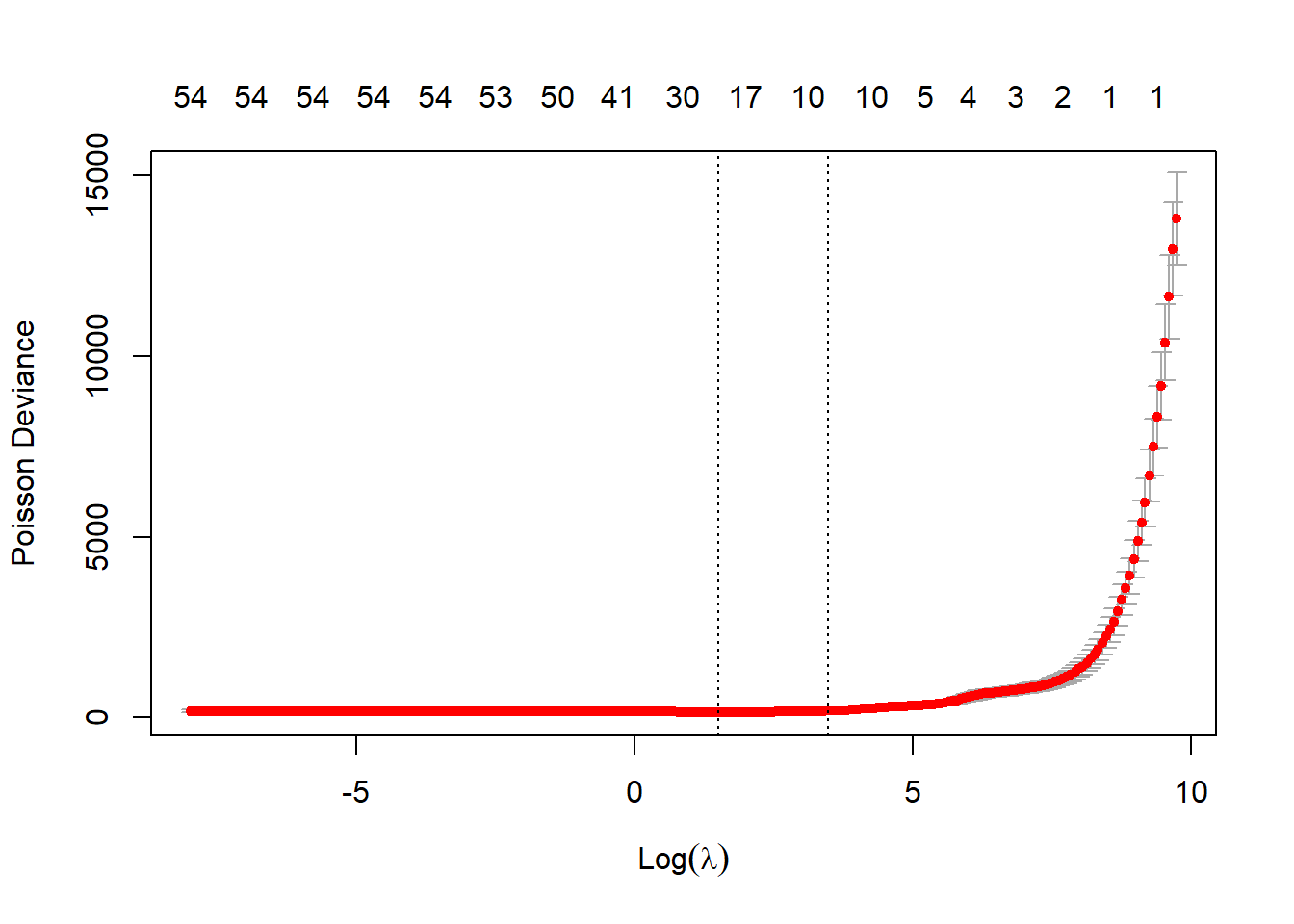
Scale parameter
Now we have a set of models and a main model in that corresponding to the lambda.1se value, we can now estimate a scale parameter assuming a gamma distribution. We do this by fitting a gamma GLM to the lambda.1se model structure and taking the scale parameter from that.
As a minor technical point, we use MASS::gamma.shape() to get the scale parameter estimate rather than that from glm() directly. This is discussed further here.
# coefficients in lambda.1se model
coefs <- predict(list_primary$glmnet_obj, type = "coefficients", s = list_primary$glmnet_obj[[main_model]])
coefnames <- c("Intercept", colnames(list_primary$varset$past))

# extract the non-zero coefficients
ind_nz_coefs <- which(!(coefs == 0))
nz_coefs <- coefs[ind_nz_coefs]
nz_coefnames <- coefnames[ind_nz_coefs]

# get the past_varset with just these observations
past_varset_small <- list_primary$varset$past[, nz_coefnames[-1]]   # the -1 removes the intercept
glm_data = as.data.table(cbind(dt[past_ind==TRUE, .(pmts)], past_varset_small))

glm_formula = as.formula(paste("pmts~", paste(nz_coefnames[-1], collapse = "+")))


#glm_formula
gamma_mod_1 = glm(formula=glm_formula, family = Gamma(link="log"), data = glm_data)

summary(gamma_mod_1)
Call:
glm(formula = glm_formula, family = Gamma(link = "log"), data = glm_data)

Deviance Residuals:
      Min         1Q     Median         3Q        Max
-0.136693  -0.048222   0.001886   0.041310   0.142041

Coefficients:
            Estimate Std. Error t value             Pr(>|t|)
(Intercept) 10.65861    0.03428 310.959 < 0.0000000000000002 ***
L_1_999_acc  0.28652    0.03021   9.485     0.00000000000266 ***
L_4_999_acc -0.19576    0.11254  -1.739              0.08879 .
L_5_999_acc -0.13971    0.18239  -0.766              0.44768
L_6_999_acc -0.01031    0.20091  -0.051              0.95930
L_7_999_acc -0.18356    0.15684  -1.170              0.24801
L_1_999_dev -0.50158    0.08647  -5.801     0.00000061660403 ***
L_2_999_dev -0.71488    0.14832  -4.820     0.00001672460156 ***
L_3_999_dev  0.27983    0.10398   2.691              0.00996 **
L_6_999_dev  0.38128    0.05998   6.356     0.00000009220787 ***
---
Signif. codes:  0 '***' 0.001 '**' 0.01 '*' 0.05 '.' 0.1 ' ' 1

(Dispersion parameter for Gamma family taken to be 0.005763095)

    Null deviance: 36.19257  on 54  degrees of freedom
Residual deviance:  0.26121  on 45  degrees of freedom
AIC: 967.87

Number of Fisher Scoring iterations: 4
Extract the updated scale parameter estimate
list_primary$scale <- round(summary(gamma_mod_1, dispersion = MASS::gamma.dispersion(gamma_mod_1))$dispersion, 4)

print(list_primary$scale)
[1] 0.0047Forecasts and residuals
- Calculate forecasts under both lambda.min and lambda.1se models and add these to
list_primary$data - Make pred field from the main model (currently lambda.1se)
- Calculate Pearson residuals
# add predictions under the two models for the min, 1se lambda values
list_primary$data[, lambda.1se := predict(list_primary$glmnet_obj, newx = list_primary$varset$all, type="response", s="lambda.1se")]
list_primary$data[, lambda.min := predict(list_primary$glmnet_obj, newx = list_primary$varset$all, type="response", s="lambda.min")]


# make pred = selected model, pred will be used later in bootstrapping
# calculate residuals - (actual - expected)/stdev
list_primary$data[, pred := get(main_model)]  # duplicate for convenience
list_primary$data[past_ind == TRUE, var_pred := (pred^2)*(list_primary$scale)
                  ][past_ind == TRUE, resid := (pmts - pred)/sqrt(var_pred)]


# also calculate reserve values
list_primary$reserves <- vector(mode="list", length = 3)
names(list_primary$reserves) <- c("primary", "lambda.1se", "lambda.min")

# lambda.1se
list_primary$reserves$lambda.1se <- list_primary$data[past_ind==FALSE, sum(lambda.1se)]
# lambda.min
list_primary$reserves$lambda.min <- list_primary$data[past_ind==FALSE, sum(lambda.min)]
# selected aka primary
list_primary$reserves$primary <- list_primary$reserves[[main_model]]

# look at reserves
as.data.table(list_primary$reserves)  |>
  datatable()  |>
  formatRound(names(list_primary$reserves), digits=0)
So the reserve under our main model is 368121 - for reference our final estimate in the CAS monograph work was $370,493.
Model diagnostics
p1 <- ggplot(data=list_primary$data[past_ind==TRUE,], aes(x=log(pred), y=resid, colour=dev)) +
    geom_point(size=2) +
    scale_colour_viridis(begin=0.9, end=0) +
    theme(legend.position = "none") +
    ggtitle("Linear predictor")


p2 <- ggplot(data=list_primary$data[past_ind==TRUE,], aes(x=acc, y=resid)) +
    geom_point(size=2, colour=me_colours$blue) +
    ggtitle("Accident")

p3 <- ggplot(data=list_primary$data[past_ind==TRUE,], aes(x=dev, y=resid)) +
    geom_point(size=2, colour=me_colours$blue) +
    ggtitle("Development")

p4 <- ggplot(data=list_primary$data[past_ind==TRUE,], aes(x=cal, y=resid)) +
    geom_point(size=2, colour=me_colours$blue) +
    ggtitle("Calendar")

(p1 + p2) / (p3 + p4)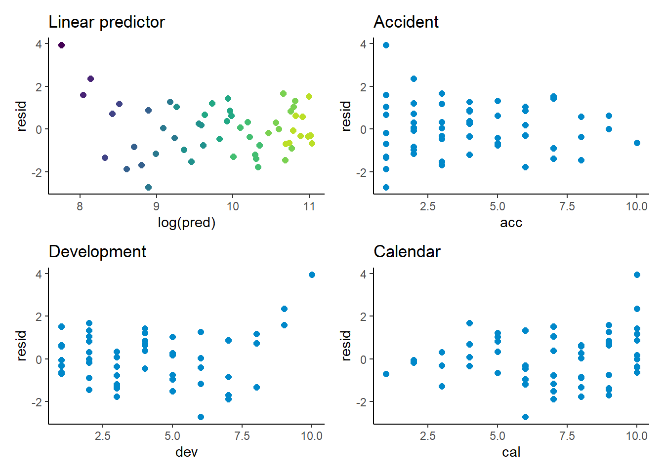
Have a look at the density plot of residuals too
ggplot(data=list_primary$data[past_ind==TRUE]) +
  geom_density(aes(resid, after_stat(density)), fill=me_colours$blue, colour=me_colours$blue) +
stat_function(fun = dnorm, colour=me_colours$orange, linewidth=2) 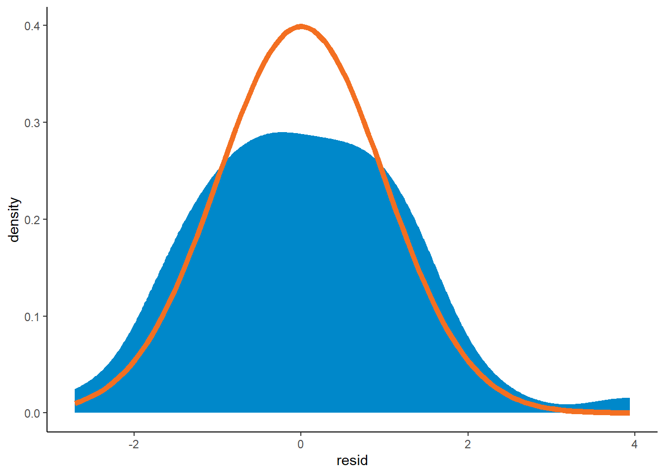
This plots shaded actual/expected values where white is close to 100%, red is where actual exceed expected (capped at 200%) and blue is where actual is less than expected (cupped at 50%).
model_forecasts_long <- melt(list_primary$data,
                             measure.vars = c("lambda.1se", "lambda.min"),
                             id.vars=c("acc", "dev", "cal", "pmts"),
                             variable.name = "model",
                             value.name = "fitted")

g <- GraphHeatMap(model_forecasts_long, x="dev", y="acc", facet="model", actual="pmts", fitted="fitted",
                  xlab="Development quarter", ylab="Accident quarter")
g$graph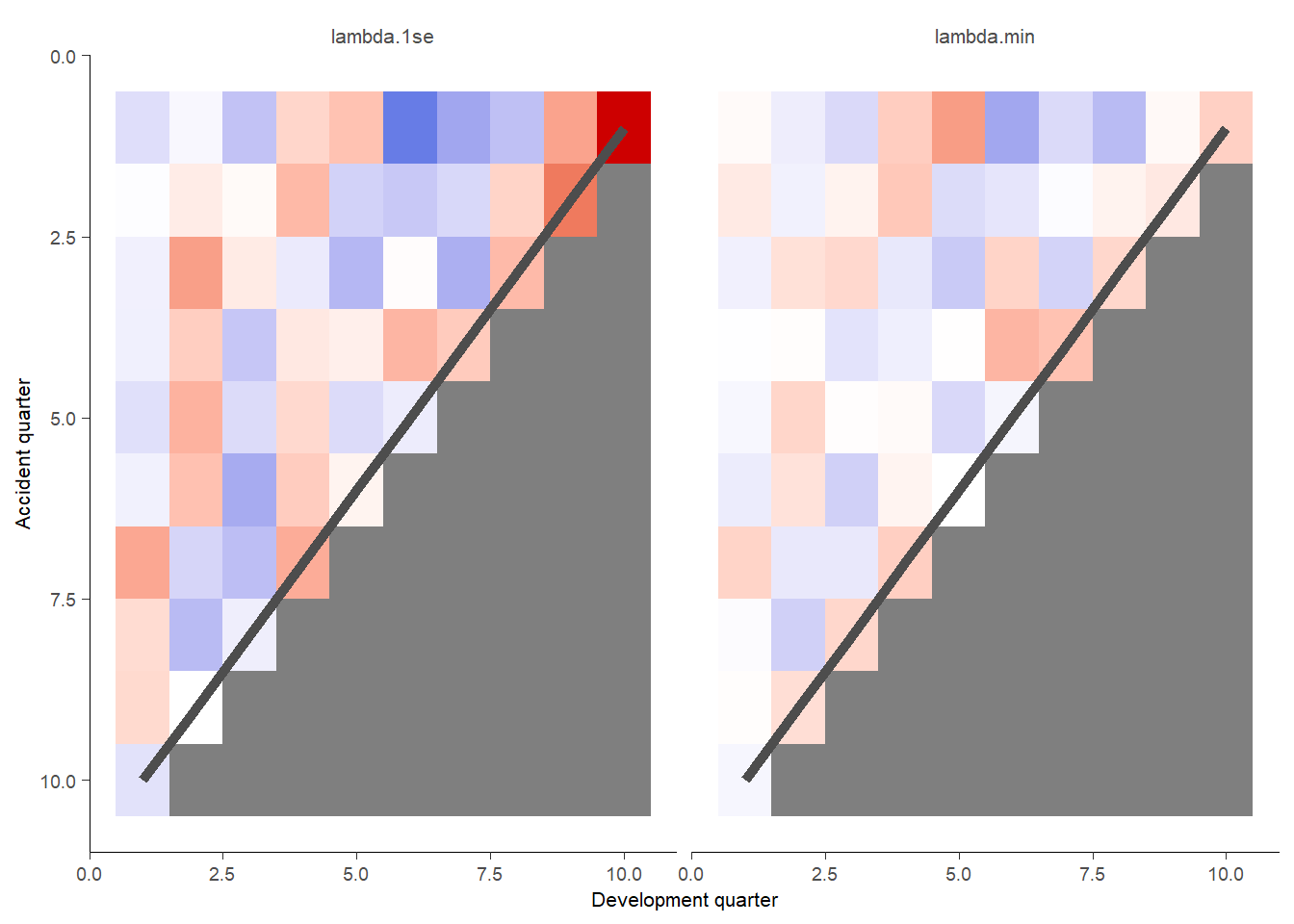
Prior
- In our paper we discuss different possibilities for priors, so refer to that discussion there
- Because the Lasso is fitted using a poisson, but our analysis assumes a gamma distribution, we need to solve for the priors that produce the desired properties, rather than use the glmnet lambda values directly
- The process is as follows:
- We specify the priors for the model parameters assuming a laplace distribution
- A fairly wide prior for the intercept term centred on the log(average past payments)
- A common scale parameter specified by us for all other coefficient and a prior mean of 0
- We then calculate the posterior distribution of each model given the laplace prior and a gamma log likelihood
- We plot the posterior distributions and select the prior values that we wish
- e.g. the prior value that leads to the lambda.1se coinciding with the posterior mode.
- We specify the priors for the model parameters assuming a laplace distribution
Filtering
As this state we should briefly discuss filtering or the inclusion gates - refer to section 5.2.5 of the paper and Table 5-1 therein as well as to the list_dt_filter_params object here.
The idea behind filtering is simple - we want to exclude models that extrapolate in a wild manner, and to an extend that an actuary would consider the model reasonable. In the paper we discussed how we looked at forecasts of different periods of payment (calendar periods) and accident periods and based the gates on that.
I have retained the same inclusion gates for this data as for the simulated data. The filtering is implemented by my CalculatePosterior() function.
Code for searching for the priors
Using a bit of trial and error and the code below, I came up with prior values for the four different types of prior considered in our paper.
The graph below won’t win any data visualisation contests, but captures the various bits and pieces of information I’ve used to interactively find the priors.
list_pp <- list(
  laplace_m_intercept = dt[past_ind==TRUE, log(mean(pmts))],   # prior mean of intercept
  laplace_s_intercept = 2,     # scale for the intercept - must be large since results not centred so intercept can be long way from data average
  laplace_m_parameters = 0,    # prior mean for the non-intercept params
  laplace_s_parameters = 0.029,
  prior_name = "finding_priors"
)

dt_post <- CalculatePosterior(list_primary$data,
                              glmnet_obj = list_primary$glmnet_obj,
                              varset = list_primary$varset$all,
                              yvar = "pmts",
                              dt_scaling_factor = NULL,
                              list_filter = list_dt_filter_params$main,
                              list_prior_params = list_pp,
                              prior_name = NULL,
                              scale = list_primary$scale)$probs


# plot ----;
# first get some quantities to put on the plot that we use in search for priors
mn_1se <- list_primary$glmnet_obj$index[rownames(list_primary$glmnet_obj$index) == "1se"]
mn_min <- list_primary$glmnet_obj$index[rownames(list_primary$glmnet_obj$index) == "min"]
mn_max_post <- dt_post[which(dt_post$posterior == max(dt_post$posterior)), model_num]
max_post <- dt_post[which(dt_post$posterior == max(dt_post$posterior)), posterior]  # used for drawing lines on graph
sum_prob_ge_1se <- round(dt_post[model_num >= mn_1se, sum(posterior)], 5)
sum_prob_le_min <- round(dt_post[model_num <= mn_min, sum(posterior)], 5)
sum_prob_ge_1se_label <- paste("Pr(>= 1se) = ", sum_prob_ge_1se, "\nso", 1-sum_prob_ge_1se, "in shaded area")
sum_prob_le_min_label <- paste("Pr(<= min) = ", sum_prob_le_min, "\nso", 1-sum_prob_le_min, "in shaded area")


ggplot(data = dt_post, mapping = aes(x = model_num, y = posterior)) +
  # max post line
  annotate("segment", x = mn_max_post, xend = mn_max_post, y=0, yend = max_post, colour = me_colours$teal, linewidth=1.5, linetype = 2) +
  annotate("text", x = mn_max_post, y = 1*max_post/3, label=paste("Max posterior model"), colour = me_colours$teal) +
  # 1se shaded box
  annotate("rect", xmin = min(dt_post$model_num), xmax = mn_1se, ymin = 0, ymax = max_post, fill = me_colours$orange, alpha = 0.1)+
  annotate("text", x = min(dt_post$model_num), y = 5*max_post/6, label=sum_prob_ge_1se_label, colour = me_colours$orange, hjust = 0) +
  # min shaded box
  annotate("rect", xmin = mn_min, xmax = max(dt_post$model_num), ymin = 0, ymax = max_post, fill = me_colours$red, alpha = 0.1)+
  annotate("text", x = max(dt_post$model_num) + 2, y = 5*max_post/6, label=sum_prob_le_min_label, colour = me_colours$red, hjust = 1) +
  # 1se line
  annotate("segment", x = mn_1se, xend = mn_1se, y=0, yend = max_post, colour = me_colours$orange) +
  annotate("text", x = mn_1se, y = 2*max_post/3, label=paste("lambda.1se model"), colour = me_colours$orange) +
  # min line
  annotate("segment", x = mn_min, xend = mn_min, y=0, yend = max_post, colour = me_colours$red) +
  annotate("text", x = mn_min, y = max_post/2, label=paste("lambda.min model"), colour = me_colours$red) +
  # posterior
  geom_line(colour = me_colours$blue) +
  labs(title = paste("Selecting prior - laplace scale is", list_pp$laplace_s_parameters),
       subtitle = paste("Max post = 1se:", mn_max_post == mn_1se, "\nMax post = min:", mn_max_post == mn_min)) +
  # coord_cartesian(xlim=c(50, 150))+   # can use this to zoom in on parts of the graph
  NULL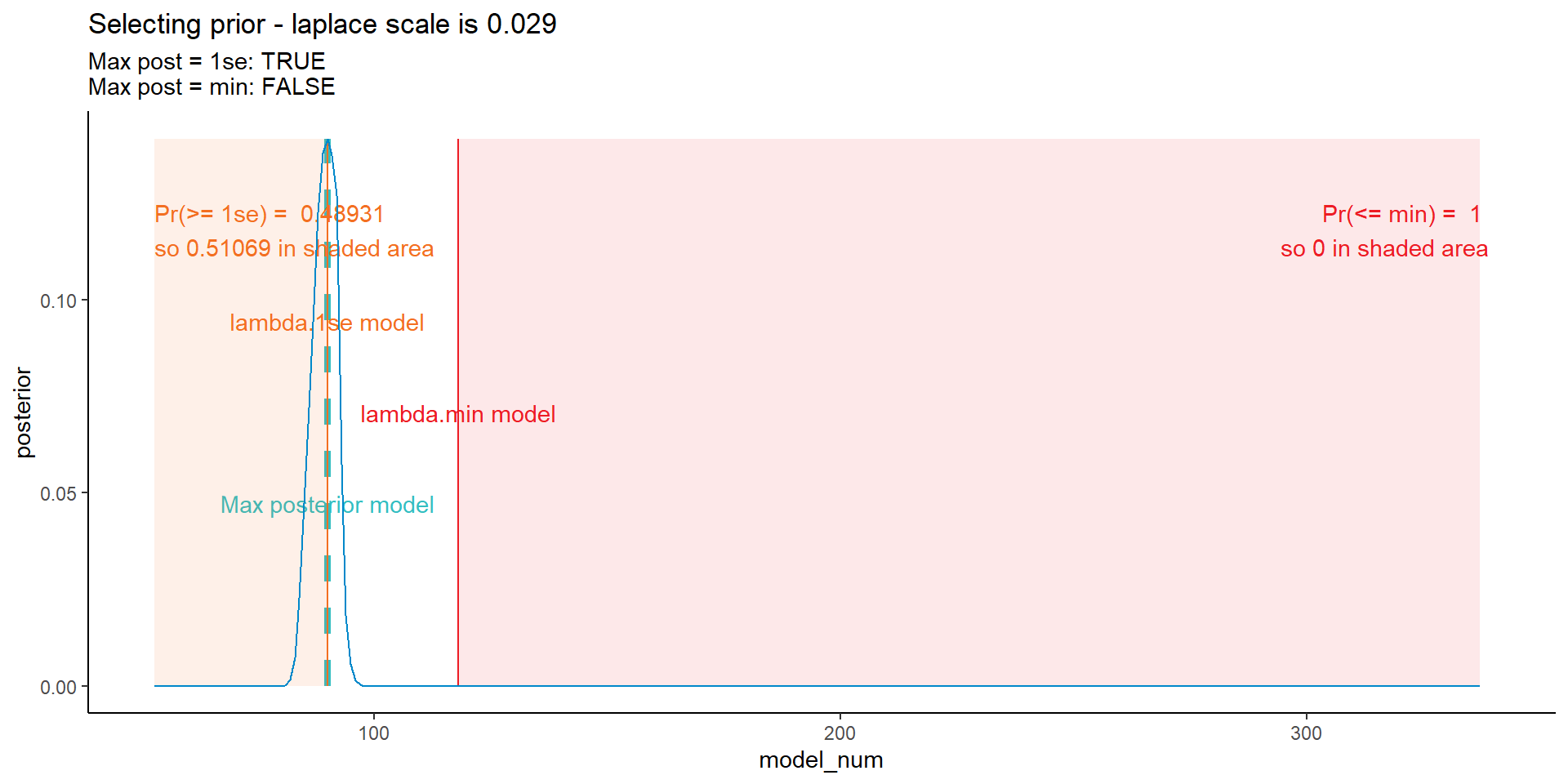
Using the code chunk above, I’ve found the priors corresponding to those used in our paper.
list_primary$prior$list_prior_params <- list(
  laplace_m_intercept = dt[past_ind==TRUE, log(mean(pmts))],   # prior mean of intercept
  laplace_s_intercept = 2,     # scale for the intercept - must be large since results not centred so intercept can be long way from data average
  laplace_m_parameters = 0,    # prior mean for the non-intercept params
  laplace_s_parameters = c(0.01505, 0.029, 0.38, 1.55),
  prior_name = c("simple", "lambda.1se", "lambda.min", "complex")
)
Posterior distributions
I’ve shown all four prior possibilities here, but later on will mainly focus on the results relating to the lambda.1se results.
Code
dt_post <- CalculatePosterior(list_primary$data,
                         glmnet_obj = list_primary$glmnet_obj,
                         varset = list_primary$varset$all,
                         yvar = "pmts",
                         dt_scaling_factor = NULL,
                         list_filter = list_dt_filter_params$main,
                         list_prior_params = list_primary$prior$list_prior_params,
                         prior_name = "simple",
                         scale = list_primary$scale)$probs


# plot ----;
# first get some quantities to put on the plot that we use in search for priors
mn_1se <- list_primary$glmnet_obj$index[rownames(list_primary$glmnet_obj$index) == "1se"]
mn_min <- list_primary$glmnet_obj$index[rownames(list_primary$glmnet_obj$index) == "min"]
mn_max_post <- dt_post[which(dt_post$posterior == max(dt_post$posterior)), model_num]
max_post <- dt_post[which(dt_post$posterior == max(dt_post$posterior)), posterior]  # used for drawing lines on graph
sum_prob_ge_1se <- round(dt_post[model_num >= mn_1se, sum(posterior)], 5)
sum_prob_le_min <- round(dt_post[model_num <= mn_min, sum(posterior)], 5)
sum_prob_ge_1se_label <- paste("Pr(>= 1se) = ", sum_prob_ge_1se)
sum_prob_le_min_label <- paste("Pr(<= min) = ", sum_prob_le_min)
pval <- list_primary$prior$list_prior_params$laplace_s_parameters[which(list_primary$prior$list_prior_params$prior_name == dt_post[1, prior_name])]

ggplot(data = dt_post, mapping = aes(x = model_num, y = posterior)) +
  # max post line
  # annotate("segment", x = mn_max_post, xend = mn_max_post, y=0, yend = max_post, colour = me_colours$teal, linewidth=1.5, linetype = 2) +
  # annotate("text", x = mn_max_post, y = 1*max_post/3, label=paste("Max posterior model"), colour = me_colours$teal) +
  # 1se shaded box
  annotate("rect", xmin = min(dt_post$model_num), xmax = mn_1se, ymin = 0, ymax = max_post, fill = me_colours$orange, alpha = 0.1)+
  annotate("text", x = min(dt_post$model_num), y = 5*max_post/6, label=sum_prob_ge_1se_label, colour = me_colours$orange, hjust = 0) +
  # min shaded box
  # annotate("rect", xmin = mn_min, xmax = max(dt_post$model_num), ymin = 0, ymax = max_post, fill = me_colours$red, alpha = 0.1)+
  # annotate("text", x = max(dt_post$model_num) + 2, y = 5*max_post/6, label=sum_prob_le_min_label, colour = me_colours$red, hjust = 1) +
  # 1se line
  annotate("segment", x = mn_1se, xend = mn_1se, y=0, yend = max_post, colour = me_colours$orange) +
  annotate("text", x = mn_1se, y = 2*max_post/3, label=paste("lambda.1se model"), colour = me_colours$orange) +
  # min line
  annotate("segment", x = mn_min, xend = mn_min, y=0, yend = max_post, colour = me_colours$red) +
  annotate("text", x = mn_min, y = max_post/2, label=paste("lambda.min model"), colour = me_colours$red) +
  # posterior
  geom_line(colour = me_colours$blue) +
  labs(title = paste(dt_post[1, prior_name], "prior - laplace scale is", pval))+
  coord_cartesian(xlim = c(50, 150)) +
  NULL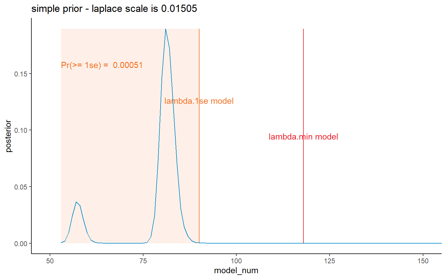
Code
dt_post <- CalculatePosterior(list_primary$data,
                         glmnet_obj = list_primary$glmnet_obj,
                         varset = list_primary$varset$all,
                         yvar = "pmts",
                         dt_scaling_factor = NULL,
                         list_filter = list_dt_filter_params$main,
                         list_prior_params = list_primary$prior$list_prior_params,
                         prior_name = "lambda.1se",
                         scale = list_primary$scale)$probs


# plot ----;
# first get some quantities to put on the plot that we use in search for priors
mn_1se <- list_primary$glmnet_obj$index[rownames(list_primary$glmnet_obj$index) == "1se"]
mn_min <- list_primary$glmnet_obj$index[rownames(list_primary$glmnet_obj$index) == "min"]
mn_max_post <- dt_post[which(dt_post$posterior == max(dt_post$posterior)), model_num]
max_post <- dt_post[which(dt_post$posterior == max(dt_post$posterior)), posterior]  # used for drawing lines on graph
sum_prob_ge_1se <- round(dt_post[model_num >= mn_1se, sum(posterior)], 5)
sum_prob_le_min <- round(dt_post[model_num <= mn_min, sum(posterior)], 5)
sum_prob_ge_1se_label <- paste("Pr(>= 1se) = ", sum_prob_ge_1se)
sum_prob_le_min_label <- paste("Pr(<= min) = ", sum_prob_le_min)
pval <- list_primary$prior$list_prior_params$laplace_s_parameters[which(list_primary$prior$list_prior_params$prior_name == dt_post[1, prior_name])]

ggplot(data = dt_post, mapping = aes(x = model_num, y = posterior)) +
  # max post line
  annotate("segment", x = mn_max_post, xend = mn_max_post, y=0, yend = max_post, colour = me_colours$teal, linewidth=1.5, linetype = 2) +
  annotate("text", x = mn_max_post, y = 1*max_post/3, label=paste("Max posterior model"), colour = me_colours$teal) +
  # 1se shaded box
  # annotate("rect", xmin = min(dt_post$model_num), xmax = mn_1se, ymin = 0, ymax = max_post, fill = me_colours$orange, alpha = 0.1)+
  # annotate("text", x = min(dt_post$model_num), y = 5*max_post/6, label=sum_prob_ge_1se_label, colour = me_colours$orange, hjust = 0) +
  # min shaded box
  # annotate("rect", xmin = mn_min, xmax = max(dt_post$model_num), ymin = 0, ymax = max_post, fill = me_colours$red, alpha = 0.1)+
  # annotate("text", x = max(dt_post$model_num) + 2, y = 5*max_post/6, label=sum_prob_le_min_label, colour = me_colours$red, hjust = 1) +
  # 1se line
  annotate("segment", x = mn_1se, xend = mn_1se, y=0, yend = max_post, colour = me_colours$orange) +
  annotate("text", x = mn_1se, y = 2*max_post/3, label=paste("lambda.1se model"), colour = me_colours$orange) +
  # min line
  annotate("segment", x = mn_min, xend = mn_min, y=0, yend = max_post, colour = me_colours$red) +
  annotate("text", x = mn_min, y = max_post/2, label=paste("lambda.min model"), colour = me_colours$red) +
  # posterior
  geom_line(colour = me_colours$blue) +
  labs(title = paste(dt_post[1, prior_name], "prior - laplace scale is", pval))+
  coord_cartesian(xlim = c(50, 150)) +
  NULL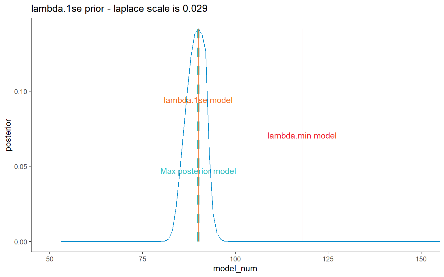
Code
dt_post <- CalculatePosterior(list_primary$data,
                         glmnet_obj = list_primary$glmnet_obj,
                         varset = list_primary$varset$all,
                         yvar = "pmts",
                         dt_scaling_factor = NULL,
                         list_filter = list_dt_filter_params$main,
                         list_prior_params = list_primary$prior$list_prior_params,
                         prior_name = "lambda.min",
                         scale = list_primary$scale)$probs


# plot ----;
# first get some quantities to put on the plot that we use in search for priors
mn_1se <- list_primary$glmnet_obj$index[rownames(list_primary$glmnet_obj$index) == "1se"]
mn_min <- list_primary$glmnet_obj$index[rownames(list_primary$glmnet_obj$index) == "min"]
mn_max_post <- dt_post[which(dt_post$posterior == max(dt_post$posterior)), model_num]
max_post <- dt_post[which(dt_post$posterior == max(dt_post$posterior)), posterior]  # used for drawing lines on graph
sum_prob_ge_1se <- round(dt_post[model_num >= mn_1se, sum(posterior)], 5)
sum_prob_le_min <- round(dt_post[model_num <= mn_min, sum(posterior)], 5)
sum_prob_ge_1se_label <- paste("Pr(>= 1se) = ", sum_prob_ge_1se)
sum_prob_le_min_label <- paste("Pr(<= min) = ", sum_prob_le_min)
pval <- list_primary$prior$list_prior_params$laplace_s_parameters[which(list_primary$prior$list_prior_params$prior_name == dt_post[1, prior_name])]

ggplot(data = dt_post, mapping = aes(x = model_num, y = posterior)) +
  # max post line
  annotate("segment", x = mn_max_post, xend = mn_max_post, y=0, yend = max_post, colour = me_colours$teal, linewidth=1.5, linetype = 2) +
  annotate("text", x = mn_max_post, y = 1*max_post/3, label=paste("Max posterior model"), colour = me_colours$teal) +
  # 1se shaded box
  # annotate("rect", xmin = min(dt_post$model_num), xmax = mn_1se, ymin = 0, ymax = max_post, fill = me_colours$orange, alpha = 0.1)+
  # annotate("text", x = min(dt_post$model_num), y = 5*max_post/6, label=sum_prob_ge_1se_label, colour = me_colours$orange, hjust = 0) +
  # min shaded box
  # annotate("rect", xmin = mn_min, xmax = max(dt_post$model_num), ymin = 0, ymax = max_post, fill = me_colours$red, alpha = 0.1)+
  # annotate("text", x = max(dt_post$model_num) + 2, y = 5*max_post/6, label=sum_prob_le_min_label, colour = me_colours$red, hjust = 1) +
  # 1se line
  annotate("segment", x = mn_1se, xend = mn_1se, y=0, yend = max_post, colour = me_colours$orange) +
  annotate("text", x = mn_1se, y = 2*max_post/3, label=paste("lambda.1se model"), colour = me_colours$orange) +
  # min line
  annotate("segment", x = mn_min, xend = mn_min, y=0, yend = max_post, colour = me_colours$red) +
  annotate("text", x = mn_min, y = max_post/2, label=paste("lambda.min model"), colour = me_colours$red) +
  # posterior
  geom_line(colour = me_colours$blue) +
  labs(title = paste(dt_post[1, prior_name], "prior - laplace scale is", pval))+
  coord_cartesian(xlim = c(50, 150)) +
  NULL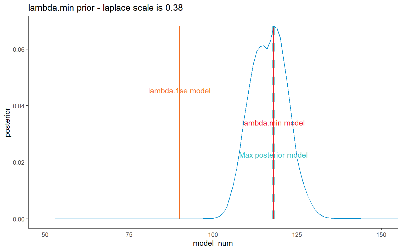
Code
dt_post <- CalculatePosterior(list_primary$data,
                         glmnet_obj = list_primary$glmnet_obj,
                         varset = list_primary$varset$all,
                         yvar = "pmts",
                         dt_scaling_factor = NULL,
                         list_filter = list_dt_filter_params$main,
                         list_prior_params = list_primary$prior$list_prior_params,
                         prior_name = "complex",
                         scale = list_primary$scale)$probs


# plot ----;
# first get some quantities to put on the plot that we use in search for priors
mn_1se <- list_primary$glmnet_obj$index[rownames(list_primary$glmnet_obj$index) == "1se"]
mn_min <- list_primary$glmnet_obj$index[rownames(list_primary$glmnet_obj$index) == "min"]
mn_max_post <- dt_post[which(dt_post$posterior == max(dt_post$posterior)), model_num]
max_post <- dt_post[which(dt_post$posterior == max(dt_post$posterior)), posterior]  # used for drawing lines on graph
sum_prob_ge_1se <- round(dt_post[model_num >= mn_1se, sum(posterior)], 5)
sum_prob_le_min <- round(dt_post[model_num <= mn_min, sum(posterior)], 5)
sum_prob_ge_1se_label <- paste("Pr(>= 1se) = ", sum_prob_ge_1se)
sum_prob_le_min_label <- paste("Pr(<= min) = ", sum_prob_le_min)
pval <- list_primary$prior$list_prior_params$laplace_s_parameters[which(list_primary$prior$list_prior_params$prior_name == dt_post[1, prior_name])]

ggplot(data = dt_post, mapping = aes(x = model_num, y = posterior)) +
  # max post line
  # annotate("segment", x = mn_max_post, xend = mn_max_post, y=0, yend = max_post, colour = me_colours$teal, linewidth=1.5, linetype = 2) +
  # annotate("text", x = mn_max_post, y = 1*max_post/3, label=paste("Max posterior model"), colour = me_colours$teal) +
  # 1se shaded box
  # annotate("rect", xmin = min(dt_post$model_num), xmax = mn_1se, ymin = 0, ymax = max_post, fill = me_colours$orange, alpha = 0.1)+
  # annotate("text", x = min(dt_post$model_num), y = 5*max_post/6, label=sum_prob_ge_1se_label, colour = me_colours$orange, hjust = 0) +
  # min shaded box
  annotate("rect", xmin = mn_min, xmax = max(dt_post$model_num), ymin = 0, ymax = max_post, fill = me_colours$red, alpha = 0.1)+
  annotate("text", x = max(dt_post$model_num) + 2, y = 5*max_post/6, label=sum_prob_le_min_label, colour = me_colours$red, hjust = 1) +
  # 1se line
  annotate("segment", x = mn_1se, xend = mn_1se, y=0, yend = max_post, colour = me_colours$orange) +
  annotate("text", x = mn_1se, y = 2*max_post/3, label=paste("lambda.1se model"), colour = me_colours$orange) +
  # min line
  annotate("segment", x = mn_min, xend = mn_min, y=0, yend = max_post, colour = me_colours$red) +
  annotate("text", x = mn_min, y = max_post/2, label=paste("lambda.min model"), colour = me_colours$red) +
  # posterior
  geom_line(colour = me_colours$blue) +
  labs(title = paste(dt_post[1, prior_name], "prior - laplace scale is", pval))+
  #coord_cartesian(xlim = c(75, 200)) +
  NULL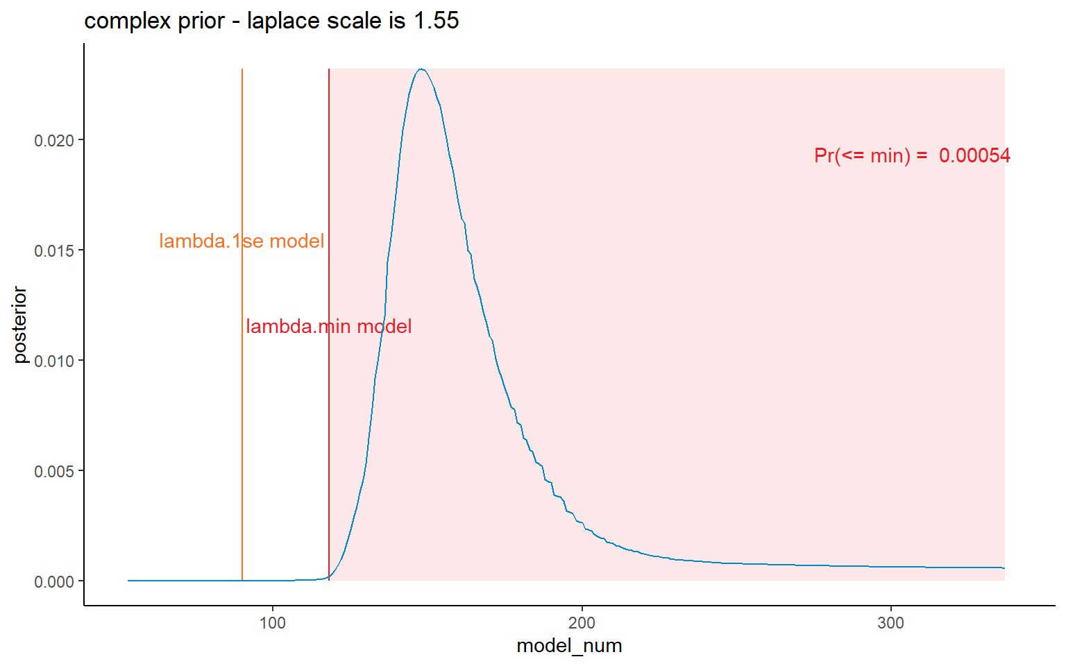
Bayesian averaging of primary model path
We get a first initial estimate of model error by applying Bayesian averaging to the Lasso model path from the initial model. We do this for each of the priors.
First get the posteriors (basically rerunning the code above but putting it into the right object this time).
list_fitted <- list_probs <- vector(mode = "list", length = length(list_primary$prior$list_prior_params$prior_name))

for(v in list_primary$prior$list_prior_params$prior_name){
  tem <- CalculatePosterior(list_primary$data,
                            glmnet_obj = list_primary$glmnet_obj,
                            varset = list_primary$varset$all,
                            yvar = "pmts",
                            dt_scaling_factor = NULL,
                            list_filter = list_dt_filter_params$main,
                            list_prior_params = list_primary$prior$list_prior_params,
                            prior_name = v,
                            scale = list_primary$scale,
                            return_fitted = TRUE)
  list_probs[[v]] <- copy(tem$probs)
  list_fitted [[v]] <- copy(tem$fitted)

}

list_primary$dt_probs <- rbindlist(list_probs)

dt_fitted <- rbindlist(list_fitted)  # needed for scaling later on

# factor prior_name to preserve ordering
list_primary$dt_probs[, prior_name := factor(prior_name, levels =list_primary$prior$list_prior_params$prior_name)]
dt_fitted[, prior_name := factor(prior_name, levels =list_primary$prior$list_prior_params$prior_name)]
Now do the Bayesian averaging. We also need to get the posterior average cashflows by acc and dev for use in the bootstraping filtering step - when applying the inclusion gates we do it relative to the posterior cashflows for that particular prior.
# run the Bayesian averaging
list_primary$dt_results <- SummariseBayesianAveraging(list_primary$dt_probs)

# Primary posterior forecasts
list_primary$dt_posterior_forecasts <- GetPosteriorForecasts(dt_fitted, list_primary$dt_probs)
Results
Finally display the results.
post_covis our initial estimate of internal model structure error - but limited since the model set is sparsepost_cov_peadds on process error (we sample each future fitted value from a gamma distribution determined by the cell mean and the scale parameter)- However this is not particularly reliable here since we don’t have enough observations.
# display table of results
list_primary$dt_results |>
  datatable() |>
  formatRound(c("post_mean", "post_sd", "post_mean_pe", "post_sd_pe"), digits=0) |>
  formatPercentage(c("post_cov", "post_cov_pe"), digits=2)
Bootstrap
Now we move onto the bootstrap. The process is described in Section 6.2 of the paper. In less formal language the steps are:
- Generate \(B\) pseudo data sets using a semi-parametric bootstrap. By this, I mean that we start with the lambda.1se fitted values, randomly sample the residuals (with replacement) \(B\) times and generate \(B\) pseudo data sets by combining the fitted values with each of the \(B\) samples
- Fit a Lasso model to each using the set of lambda values used in the primary model
- For each bootstrapped sample, produce the liability estimates and posterior probabilities. Since we will centre the bootstraps around the posterior forecasts (next point), which in turn will change the posteriors, use wider inclusion gates to avoid eliminating bootstraps on the boundary of acceptability
- Calculate the scaling factor required to scale the sample mean of the posterior means from each pseudo data set to the original posterior means
- Filter the results based on the normal inclusion gates
- Recalculate the reserves and posterior probabilities
- Drop any bootstrap replication \(b\) which has fewer than 5 models with a posterior probability of at least 0.0001.
In terms of R code, I’ve wrapped all this up in a single function (consisting of a number of other sub-functions) - ParallelBootstrap(). So you’ll need to refer to the function file for the details there.
Semi-parametric bootstrap and first round of calculations
Here we do steps 1-3 from above.
As with the primary model, we’ll make a list to hold all the results from the bootstrapping
list_bs <- list()The time-consuming part of this process is fitting the Lasso models. In the _functions.R file, the BootstrapBatch() is the actual workhorse function that does the bootstrapping. ParallelBootstrap() is a wrapper around it which gives the option of running the code in parallel to speed things up. For example, to produce the numerical results in the paper, I ran 10 parallel processes on a linux machine and it took about 72 minutes.
Note that the parallelisation currently only works on linux since I’ve used forking. If you want to run parallel code under windows you will need to edit the ParallelBootstrap() function to handle sockets.
x <- ParallelBootstrap(dt = list_primary$data,
                       nboot = num_bootstraps,
                       scale = list_primary$scale,
                       resid_name = "resid",
                       var_pred_name = "var_pred",
                       min_val = 10,
                       vec_lambda = lambdavec,
                       list_varset = list_primary$varset,
                       yvar = "pmts",
                       dfmax = dfmax_default,
                       pmax = pmax_default,
                       thresh = 1e-7,  # higher threshold speeds things up a bit
                       list_prior_params = list_primary$prior$list_prior_params,
                       dt_scaling_factor = NULL,
                       list_filter = list_dt_filter_params$initial,  # wider gates
                       parallel = use_parallel,   # TRUE for parallel, only works on linux
                       nworkers = num_workers,    # set to number of parallel processes
                       batchsize = batchsize
)
[1] "Time taken: 3.7992 mins"list_bs$list_glmnet <- x$list_glmnet
list_bs$dt_unscaled_probs <- x$dt_probs
list_bs$dt_bs_data <- x$dt_bs_data
list_bs$dt_unscaled_results <- CalculateModelError(list_bs$dt_unscaled_probs, min_model_number = 5, min_model_prob_threshold = 1e-4)$results
rm(x)
gc() used (Mb) gc trigger (Mb) max used (Mb)
Ncells 2526149 135.0 4438395 237.1 4438395 237.1
Vcells 9087459 69.4 17860456 136.3 17860456 136.3ParallelBootstrap() returns a list with three elements:
- a list of all the fitted Lasso models, one for each bootstrap
- a data.table of the posterior probabilities for all the models that survive the filtering
- a data.table of all the pseudo data sets.
I’ve calculated results after this initial round. This is to facilitate the scaling (next step), other than that we don’t use these results
Scaling factors
- Calculate factors so that the posterior bootstrapped means will match the means from the primary model (step 4 above)
- Note, however, that we don’t expect to get exact matches after scaling. This is because the scaling will lead to some changes in the posterior calculations, and possibly even the included bootstraps
# combine bootstrap means and primary posterior means and get scaling
list_bs$dt_scaling <- list_bs$dt_unscaled_results[ list_primary$dt_results[, .(prior_name, post_mean)],
                                          on=.(prior_name),
                                          primary_post_mean := i.post_mean][, .(prior_name, primary_post_mean, bs_means_mean)]

list_bs$dt_scaling[, scaling_factor := primary_post_mean / bs_means_mean]

# print out the scaling factors
list_bs$dt_scaling |>
  datatable() |>
  formatRound(columns = c("bs_means_mean", "primary_post_mean"), digits=0, mark=",") |>
  formatPercentage(columns = c("scaling_factor", "scaling_factor"), digits=2)
Rescale the bootstraps
We now carry out steps 5-7 above. When calling ParallelBootstrap() this time:
- The input data is the data.table containing all the pseudo data sets
- I use the argument
list_glmnetto pass in the list of fitted Lassos. This tells the function not to actually refit the Lasso models. Instead, it just scales the past fitted values for the scaling factor (for the likelihood) and adjusts the intercept term in all the models by the scaling factor (for the prior and the reserve predictions). - I also use the main inclusion gates rather than the wider ones.
The function then carried out steps 5-7 and we get a table of all retained bootstraps and the posterior probability of each model. We can then calculate the model error with the CalculateModelError() function.
x <- ParallelBootstrap(dt = list_bs$dt_bs_data,
                       nboot = num_bootstraps,
                       scale = list_primary$scale,
                       resid_name = "resid",
                       var_pred_name = "var_pred",
                       min_val = 10,
                       vec_lambda = lambdavec,
                       list_varset = list_primary$varset,
                       yvar = "pmts",
                       dfmax = dfmax_default,
                       pmax = pmax_default,
                       thresh = 1e-7,
                       list_prior_params = list_primary$prior$list_prior_params,
                       dt_scaling_factor = list_bs$dt_scaling,
                       list_filter = list_dt_filter_params$main,
                       parallel = use_parallel,
                       nworkers = num_workers,
                       batchsize = batchsize,
                       list_glmnet = list_bs$list_glmnet )
[1] "Time taken: 2.8138 mins"list_bs$dt_probs <- x$dt_probs
tem <- CalculateModelError(list_bs$dt_probs, min_model_number = 5, min_model_prob_threshold = 1e-4)
list_bs$dt_results <- tem$results
list_bs$dt_retained_bs <- tem$retained_bs
rm(x, tem)
gc() used (Mb) gc trigger (Mb) max used (Mb)
Ncells 2526368 135.0 4438395 237.1 4438395 237.1
Vcells 9627279 73.5 21512547 164.2 17860456 136.3Results
Finally we can look at some results. I’ve shown results for all priors here, but, as per the paper, we consider the lambda.1se and the lambda.min priors the appropriate ones to choose between. In both of those all bootstraps are retained (same is true for simple), but many are filtered out for the complex model - and, based on the CDF graphs, it is inappropriate to use it.
# used to format tables

percent_cols <- c("bs_covs_mean", "bs_variances_cov", "bs_means_cov",
                  "cov_model_param_process_error", "cov_model_error", "cov_param_error", "cov_process_error")
percent_cols <- c(percent_cols, paste0(percent_cols, "_pe"))grand_results_cols <- c("cov_model_param_process_error", "cov_model_error", "cov_param_error", "cov_process_error",
"bs_means_mean", "num_bs",
"sd_model_param_process_error", "sd_model_error", "sd_param_error", "sd_process_error")
kv <- c("prior_name", grand_results_cols)
kvpc <- intersect(kv, percent_cols)
list_bs$dt_results[, ..kv] |>
datatable() |>
formatRound(columns = setdiff(kv, c("prior_name", kvpc)), digits=0, mark=",") |>
formatPercentage(columns = kvpc, digits=2) Grand results taken calculated from this
kv <- setdiff(names(list_bs$dt_results), grand_results_cols)
kvpc <- intersect(kv, percent_cols)

list_bs$dt_results[, ..kv] |>
  datatable() |>
  formatRound(columns = setdiff(kv, c("prior_name", kvpc)), digits=0, mark=",") |>
  formatPercentage(columns = kvpc, digits=2)
# calculate posterior means, variances
list_bs$dt_idv_results <- list_bs$dt_probs[,`:=`(bs_post_mean = sum(reserve * posterior), bs_post_mean_pe = sum(reserve_pe * posterior)),
by=.(boot, prior_name)
][, .(bs_post_mean = mean(bs_post_mean),
bs_post_mean_pe = mean(bs_post_mean_pe),
bs_post_var = sum( ((reserve - bs_post_mean)^2) * posterior),
bs_post_var_pe = sum( ((reserve_pe - bs_post_mean_pe)^2) * posterior) ),
keyby = .(boot, prior_name)]
# add sd and cov now
list_bs$dt_idv_results[, `:=`(bs_post_sd = sqrt(bs_post_var),
bs_post_sd_pe = sqrt(bs_post_var_pe),
bs_post_cov = sqrt(bs_post_var) / bs_post_mean,
bs_post_cov_pe = sqrt(bs_post_var_pe) / bs_post_mean_pe)]
datatable(list_bs$dt_idv_results, options = list(pageLength = 12, lengthMenu=c(12, 20, 40, 100))) |>
formatRound(columns = setdiff(names(list_bs$dt_idv_results), c("boot", "prior_name", "bs_post_cov", "bs_post_cov_pe")), digits=0, mark=",") |>
formatPercentage(columns = c("bs_post_cov", "bs_post_cov_pe"), digits=2) # probs_retained_bs calculated above
# combine the original and bootstrapped priors now
cdfs <- rbind( list_primary$dt_probs[, .(model_num, prior_name, posterior, reserve)][, boot := 0],
list_bs$dt_probs[, .(boot, model_num, prior_name, posterior, reserve)] )
setorder(cdfs, boot, prior_name, reserve)
cdfs[, cdf := cumsum(posterior), keyby=.(boot, prior_name)]
# plot
ggplot(data=cdfs, aes(x=reserve, y=cdf, colour = factor(boot), alpha = factor(boot), linewidth = factor(boot)))+
geom_line()+
facet_wrap(~prior_name)+
scale_colour_manual(values=c(me_colours$red, rep(me_colours$grey, max(cdfs$boot))))+
scale_alpha_manual(values=c(1, rep(0.25, max(cdfs$boot))))+
scale_linewidth_manual(values=c(2, rep(0.5, max(cdfs$boot))))+
scale_x_continuous(labels = label_number(scale_cut = cut_short_scale()))+
theme(legend.position="none")+
NULL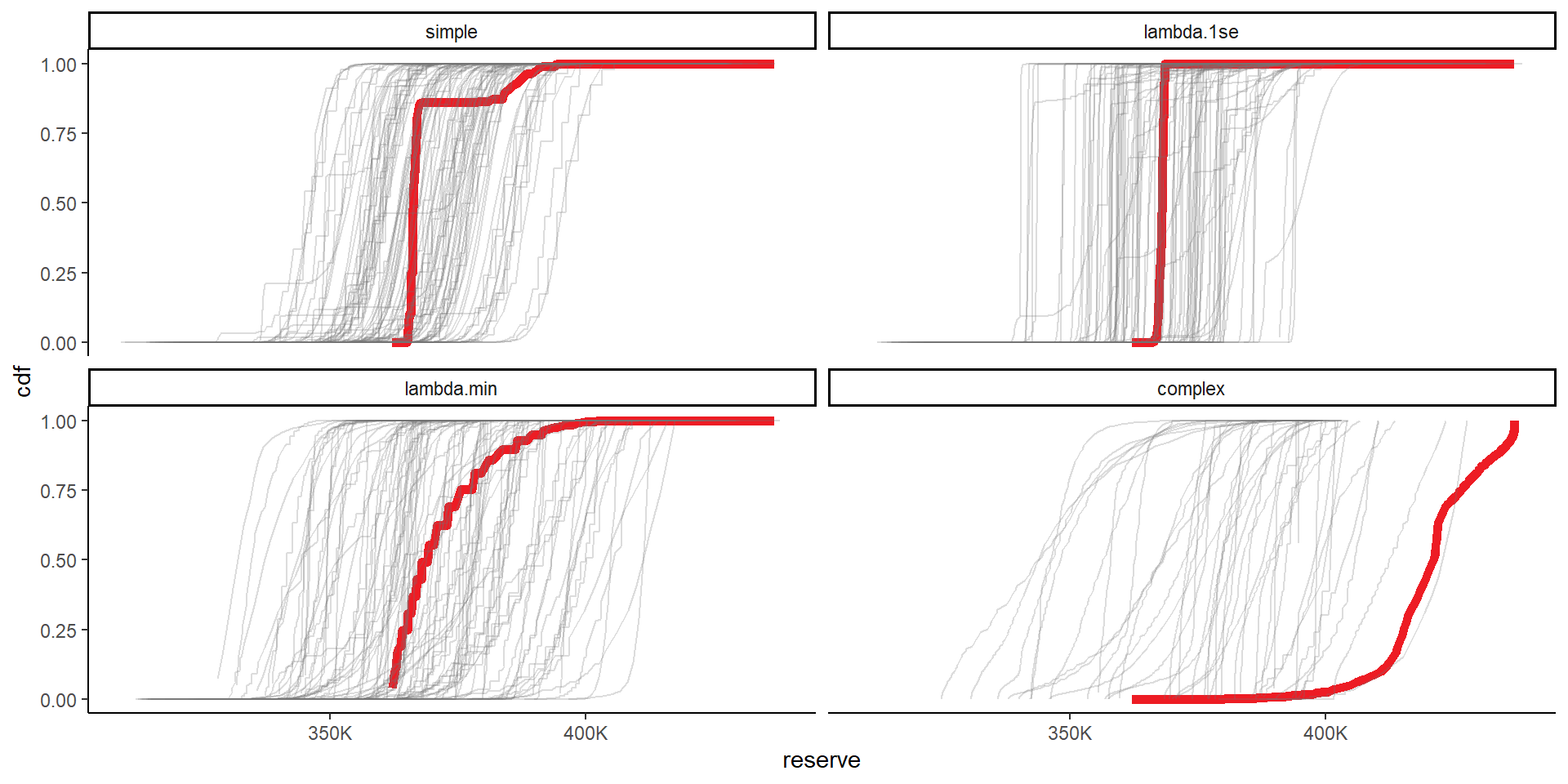
# probs_retained_bs calculated above

# combine the original and bootstrapped priors now
cdfs <- rbind( list_primary$dt_probs[, .(model_num, prior_name, posterior, reserve)][, boot := 0],
               list_bs$dt_probs[, .(boot, model_num, prior_name, posterior, reserve_pe)][, reserve := reserve_pe][, reserve_pe := NULL]  )

setorder(cdfs, boot, prior_name, reserve)
cdfs[, cdf := cumsum(posterior), keyby=.(boot, prior_name)]

# plot
ggplot(data=cdfs, aes(x=reserve, y=cdf, colour = factor(boot), alpha = factor(boot), linewidth = factor(boot)))+
  geom_line()+
  facet_wrap(~prior_name)+
  scale_colour_manual(values=c(me_colours$red, rep(me_colours$grey, max(cdfs$boot))))+
  scale_alpha_manual(values=c(1, rep(0.25, max(cdfs$boot))))+
  scale_linewidth_manual(values=c(2, rep(0.5, max(cdfs$boot))))+
  scale_x_continuous(labels = label_number(scale_cut = cut_short_scale()))+
  theme(legend.position="none")+
  NULL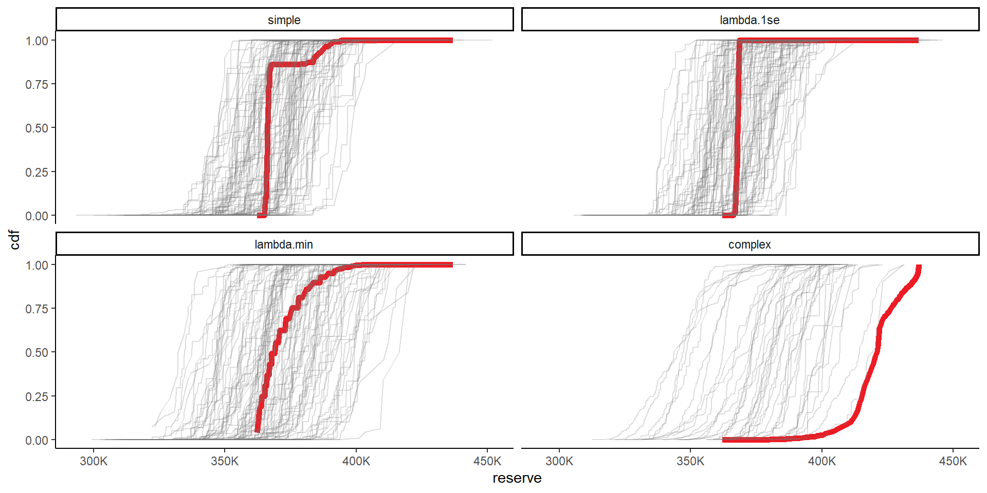
Comparison with previous results
In Section 5.4.2 of the CAS monograph, we used the bootstrap to estimate parameter and process error and found a coefficient of variation of prediction of 3.8%.
Our results for the two main priors are 3.5% and 5.1% so in a similar ball-park. A priori we’d expect low internal model structural error for this data set since we know that it is well represented by a chain ladder model, while a small number of interactions improve it further. It’s also quite small and simple so we can be confidence that we’re not missing model structure.
The GLM results in the monograph were not subject to any filtering of results for inappropriate extrapolation so may have slightly overstated parameter and process error. As noted in our paper (Section 7.4), results can be quite sensitive to inclusion gates.
Conclusion
In this tutorial we’ve worked through the our forecast error estimation process. The same code can be used for larger data sets, such as the synthetic data sets from the paper, with the relevant adjustments (mainly high-level stuff, e.g. appropriate parameters for creating the basis functions).
While some of this functionality is specific to models fitted with a Lasso (e.g. prior specification and selection), other parts (e.g. the filtering) are of relevance to any bootstrapping exercise, whether underpinned by a machine learning algorithm, a GLM or even a chain ladder.
Finally, don’t forget about the other components of forecast error, specifically external model error, which may require other, more qualitative methods to assess.